
RESEARCH ARTICLE
A Simulation Study to Evaluate Survey Designs and Assessment Models for Estimation of Dungeness Crab (Cancer magister) Softshell Periods
Zane Zhang*, Jason S. Dunham
Article Information

Identifiers and Pagination:
Year: 2016Volume: 9
First Page: 57
Last Page: 74
Publisher Id: TOFISHSJ-9-57
DOI: 10.2174/1874401X01609010057
Article History:
Received Date: 21/07/2016Revision Received Date: 02/09/2016
Acceptance Date: 21/10/2016
Electronic publication date: 27/12/2016
Collection year: 2016
open-access license: This is an open access article licensed under the terms of the Creative Commons Attribution-Non-Commercial 4.0 International Public License (CC BY-NC 4.0) (https://creativecommons.org/licenses/by-nc/4.0/legalcode), which permits unrestricted, non-commercial use, distribution and reproduction in any medium, provided the work is properly cited.
Abstract
Softshell Dungeness Crabs have inferior meat quality and are vulnerable to handling by harvesters; therefore, knowing when softshell periods occur is important for managing Dungeness Crab fisheries. A computer simulation was used to study the effectiveness of several survey designs and statistical models for estimating softshell periods which normally would be construed from crab shell condition data obtained from trap surveys. Survey designs varied in the number of years of data collection (1, 3, 5 or 10 years) and by the number and arrangement of sampling events per year. Three statistical models, including standardized catch-per-unit-effort (SCPUE), hierarchical, and generalized additive, were tested using catch-per-unit-effort data (CPUEs) or CPUE- transformed data. CPUEs were standardised by dividing CPUE estimates by the maximum CPUE obtained in the sample year, and then transformed using the complementary log-log function. In the hierarchical model, CPUEs were modelled using a lognormal distribution, assuming the expected logarithms of CPUEs are a quadratic function of days plus a random normal error. CPUE-transformed data were modelled using a normal distribution, assuming expected values are a quadratic function of days in the SCPUE model or a spline smooth function of days in the generalized additive model. Results suggest the best survey design requires a relatively high number (6 or 11) of sampling events during several key consecutive months which contain the softshell period, and fewer sampling events during those months when softshell crab abundance is low. A minimum 3 years of data collection is required to produce reliable outputs. The hierarchical model performs best, slightly better than the SCPUE model. Use of the generalized additive model is not recommended.
1. INTRODUCTION
Dungeness Crabs (Cancer magister) are distributed from California to Alaska and inhabit the open ocean along the west coast of North America and inland marine waters [1, 2]. Large males are targeted by commercial, recreation, and First Nations trap fisheries. Dungeness Crabs grow by moulting, a process whereby a new soft shell is formed and the old hard shell is shed. Newly moulted crab shells harden in 2-3 months [3, 4]; during this time, however, the quality and marketability of crab meat is negatively affected [5] and crabs are vulnerable to handling injuries [6-8]. For these reasons harvest restrictions, including fishery closures and trap haul restrictions, have been implemented by managers to improve the economics of fisheries and protect softshell crabs. Fishery closures are used in American crab fisheries and in three Crab Management Areas (CMAs) in British Columbia (BC): Hecate Strait/Queen Charlotte Islands (CMA A), Fraser River delta (CMA I) and Boundary Bay (CMA J). Trap haul restrictions involve limiting the number of times traps can be removed from the water during specified periods and are utilized in three CMAs in BC: along the west coast of Vancouver Island (CMA E), in Johnstone Strait (CMA G), and in the Strait of Georgia (CMA H). Hauling traps less frequently is believed to reduce handling mortality [9].
Dungeness Crabs reach sexual maturity at 2 or 3 years of age [3]. Juvenile crabs moult multiple times each year, whereas adults usually moult once per year [4, 10]. In general, adult male Dungeness Crabs moult between June and August in California, in August in Oregon, and in September in Washington following moulting of, and mating with, females in the spring (February to July) [11]. In contrast, in BC and southeast Alaska the male moult generally occurs between February and July [3, 12] prior to the female summer moult and mating period. However, moult timing seems to vary in different geographical areas, especially at smaller spatial scales, likely due to different oceanographic and hydrodynamic features [13]. For example, in Puget Sound the primary moult timing for males varies between subareas [14, 15]. In BC, the peak softshell period occurs in March along the east coast of the Strait of Georgia [9] and in May along the west coast of the strait in the Fraser River delta [16]. Moult timing is not readily known in many areas in BC, especially in the central and north coasts, and there is increasing interest from groups such as First Nations to better understand the biology of local crab populations, including moult timing of both males and females.
In BC, between 2009 and 2013, in order to determine Dungeness Crab softshell periods, contract biologists hired by industry – termed service providers – conducted fishery independent standardized trap sampling to collect crab biological data, including shell condition information, in three CMAs which are open year-round to commercial crab fishing. Surveys occurred in index sites twice each month from January to June and once per month from July to December. Statistical models were used to estimate peak softshell timing based on survey data [9]. The SCPUE model described in the Materials and Methodology section determined the abundance of legal-sized softshell crabs peaked during March. One reviewer of the manuscript suggested trying the hierarchical model which ultimately produced moderately different results, but merits of the two different models, in terms of estimation accuracies, could not be evaluated without a computer simulation test.
In this study we conducted simulation testing to investigate the effectiveness of various survey designs and statistical models, in terms of accuracy, in estimating softshell timing in male Dungeness Crabs. We also varied the number of years during which data were collected in simulations, and quantified impacts on estimation stabilities.
2. MATERIALS AND METHODOLOGY
The study by Waddell et al. (2016) revealed that abundance of legal-sized softshell male Dungeness Crabs is typically low in the late fall and early winter in the Strait of Georgia, on the west coast of Vancouver Island, and in Johnstone Strait. Abundance peaks during the spring and gradually decreases throughout the summer. We simulated similar temporal patterns of softshell crab abundance using a two-piece normal model [17]. The generated annual abundance data contained three days of particular interest: 1) the peak day when abundance was highest, 2) the lower day, a particular day prior to the peak day when abundance was 85% of the maximum, and 3) the upper day, a particular day after the peak day when abundance was 85% of the maximum. The period of time (days) between the lower and upper days is defined as the softshell period. We produced five hundred replicates of soft shell abundance data in ways as described below. Survey data were obtained from these simulated abundances using alternative survey designs in terms of the number of survey years, the number of sampling events during a particular year, and various arrangements of the timing of sampling events. The effectiveness of these survey designs was evaluated using three methods (models). Peak, lower, and upper days were compared with the corresponding ‘true’ days to quantify estimation accuracies or errors.
2.1. Generation of Simulated Abundance of Softshell Crabs
The number of softshell crabs on a particular day is the sum of newly moulted crabs and crabs that had already moulted before this day (i.e., “old softshells”). The expected number of newly moulted crabs on a given day during the year was generated using a two-piece normal distribution, which takes the left half of a normal distribution with parameters µ and σ1 and the right half with parameters µ and σ1 and gives a common value at µ:
 |
(1) |
where subscripts, y and d, represent year and day, respectively, σl and σr are two standard deviations set to be 60 and 70 respectively (Table 1), and (µ) is the day (peak day) with the maximum number
 of moulting crabs. Peak days vary between different years and the peak day for a particular year (µy) is randomly generated from a normal distribution with the mean and coefficient of variation set to be 150 and 5%, respectively (Table 1). The number of moulting crabs on the peak day also varies between years, and Фy is randomly generated from a lognormal distribution with the median and coefficient of variation set to be 1,000 and 53.3%, respectively (Table 1). Actual number for a given day and year (Ny, d) is randomly generated from a lognormal distribution with the median and coefficient of variation set to be
 and 0.31, respectively (Table 1). The number of ‘old’ softshell crabs is set to be 30 for day 1 of the first survey year. Each softshell crab, newly moulted or ‘old’, has a probability of 0.05 ceasing to be a soft shell crab the next day due to mortality or shell hardening (Table 1). Altogether 500 replicates (sets) of daily abundance of softshell crabs were randomly produced, each being 10 years long.
| Normal distribution for generating a day (µy) in a survey year when maximum moulting occurs | |
| mean | 150 |
| coefficient of variation | 0.05 |
| Lognormal distribution for generating number of moulting crabs (Фy) at day µy | |
| Median | 1000 |
| coefficient of variation | 0.53 |
| Two-piece normal distribution for generating expected number () of moulting crabs for a given day of a survey year |
|
| the maximum and common value | |
| standard deviation for the left half | 60 |
| standard deviation for the right half | 70 |
| Lognormal distribution for generating actual number (Ny, d) of moulting crabs for a given day of a survey year | |
| Median | |
| coefficient of variation | 0.31 |
| Sustaining probability for a softshell crab | 0.95 |
| Catchability coefficient | 0.0002 |
| Lognormal distribution for generating random variate for catch per unit effort | |
| Median | 1 |
| coefficient of variation | 0.59 |
2.2. Survey Designs
Surveys varied by the number of years data were collected (1, 3, 5 or 10 years) and by the number and arrangement of sampling events per year. A particular number and arrangement of sampling events is referred to as a survey scheme, which is specified by two numbers connected by a hyphen. The first number indicates the number of sampling events; the second number indicates the number of months (6 or 12) during which sampling was conducted. For example, a 12-6 sampling scheme (abbreviated S12-6) means 12 sampling events occurred within a 6-month period. When sampling took place during a 6-month period, the 6 months chosen contained the known spring softshell period. These survey schemes are termed 6-month survey schemes in contrast to 12-month survey schemes during which sampling events occurred during a 12-month period. Intervals between two consecutive sampling events were 15, 30, 45 or 60 days (Table 2).
| 6-6 | 12-6 | 6-12 | 11-12 | 12-12 | 18-12 | 24-12 |
| 15 | 15 | 15 | 15 | 15 | ||
| 30 | ||||||
| 45 | 45 | 45 | ||||
| 60 | ||||||
| 75 | 75 | 75 | 75 | 75 | ||
| 90 | 90 | 90 | ||||
| 105 | 105 | 105 | 105 | 105 | ||
| 120 | 120 | 120 | 120 | |||
| 135 | 135 | 135 | 135 | 135 | 135 | 135 |
| 150 | 150 | 150 | 150 | |||
| 165 | 165 | 165 | 165 | 165 | 165 | |
| 180 | 180 | 180 | 180 | |||
| 195 | 195 | 195 | 195 | 195 | 195 | 195 |
| 210 | 210 | 210 | 210 | |||
| 225 | 225 | 225 | 225 | 225 | ||
| 240 | 240 | 240 | ||||
| 255 | 255 | 255 | 255 | 255 | 255 | 255 |
| 270 | ||||||
| 285 | 285 | 285 | ||||
| 300 | ||||||
| 315 | 315 | 315 | 315 | 315 | ||
| 330 | ||||||
| 345 | 345 | 345 | ||||
| 360 |
Catch of softshell crabs per unit effort (CPUE) was generated from a lognormal distribution:
 |
(2) |
where the subscript t denotes a sampling day (number of days since the beginning of a year), q is a catchability coefficient set to be 0.0002, and ϕ is a random variate generated from a lognormal distribution with median and coefficient of variation set to be 1 and 0.59, respectively (Table 1).
CPUE estimates are expected to fluctuate at different sampling days of a given year as softshell crab abundance changes. Overall magnitudes of CPUEs may also vary greatly inter-annually due to variations in overall abundance of softshell crabs in different years. To retain intra-annual fluctuations in CPUEs and remove inter-annual variations in overall CPUE magnitudes, we divided each of the CPUEs obtained in a year by the maximum CPUE in that year:
 |
(3) |
SCPUE values range between 0 and 1. To convert these values to real numbers in order to apply a normal probability distribution in the modelling process, SCPUE estimates were transformed using the complementary log-log (clog-log) function:
 |
(4) |
Each survey design was independently applied 500 times on the 500 randomly simulated sets of softshell abundance. Therefore, 500 replicates of CPUE data sets were produced for each survey design.
2.3. Model Fitting Procedure
We used three different models in this study: standardized catch-per-unit-effort (SCPUE), hierarchical, and generalized additive. The first and third models used CLSU data, whereas the hierarchical model used CPUE data.
2.3.1. SCPUE Model
was modelled using a normal distribution:
 |
(5) |
where the variance, σ12, is a model parameter, and  is the model-expected clog-log transformed value for SCPUE and is assumed to be a function of t:
 |
(6) |
where α1, α2, and α3 are model parameters. The expected SCPUE for any given day (d) was calculated as:
 |
(7) |
2.3.2. Hierarchical Model
CPUE was modelled using a lognormal distribution:
 |
(8) |
where the variance, σ22, is a model parameter and  is the natural logarithm of expected CPUE and is assumed to be a function of t with a hierarchical structure:
 |
(9) |
where β1, β2, and β3 are model parameters, and ε is a random process error which has a normal distribution with a mean of 0 and variance of σ32 (a model parameter). The expected CPUE for any given day was calculated as:
 |
(10) |
2.3.3. Generalized Additive Model
CLSU was modelled using a normal distribution:
 |
(11) |
where the variance, σ42, is a model parameter and
is related to t:
 |
(12) |
where λ is an unknown intercept (model parameter), S is a spline smooth function with the amount of smoothing determined automatically in the modelling process. The package of mgcv was used to fit the additive model on the software platform of R [18].
on a given day was predicted using the function of ‘predict’ in the package of mgcv, and the expected SCPUE for the corresponding day was calculated as:
 |
(13) |
2.4. Evaluation of Model Performance
The number of softshell crabs for each day in a particular year was randomly generated for 10,000 years as described in Section 2.1. The peak, lower, and upper days were calculated for each year and their means over the 10,000 years were regarded as the ‘true’ peak, lower, and upper days.
Performances of alternative survey designs and estimation models were evaluated by comparing errors, biases, and variations between estimated peak, lower, and upper days and the ‘true’ corresponding days. An ‘error’ is defined as the difference in days between the mean for peak, lower, or upper day as estimated from one data set and the ‘true’ value for the corresponding day. There were 500 errors in estimation of the peak, lower, or upper day for each sampling scheme, as there were 500 data sets (replicates).
‘Bias’ is defined as the median of the 500 errors, and ‘absolute bias’ is the absolute value for the bias.
‘Variation’ is defined as the difference between the 95th and 5th percentiles of the 500 errors, and shows a degree of precision in the estimation.
An absolute error is the absolute value for an error, and ‘mean absolute error’ is the mean of the 500 absolute errors, signifying the combined impact of bias and variation. For example, when the amounts of two variations were the same yet biases were different, then the estimation with the lower amount of bias would have a lower absolute mean error. We also calculated the average of three absolute biases and variations or mean absolute errors for the peak, lower, and upper days for each survey design. This average is correspondingly termed ‘overall bias’, ‘overall variation’, or ‘overall error’ and was used to evaluate overall performance for estimating the three interested days (peak, lower, and upper) for a given survey design. Furthermore, we calculated the average of eight absolute biases, variations or mean absolute errors for the peak, lower, or upper day—four from survey schemes S11-12, S12-12, S18-12, and S24-12 by the SCPUE model and the other four from the same four schemes by the hierarchical model. This average is correspondingly termed ‘average absolute bias’, ‘average variation’ or ‘average absolute error’, and was used to evaluate effects from altering the number of survey years.
2.5. Bayesian Analyses
The SCPUE and hierarchical models were fitted using a Bayesian approach with WinBUGS software [19, 20]. Uninformative priors were assigned to all model parameters. α1, α2, α3, β1, β2, β3 and were each assigned a normal distribution with large variance: N(0, 1002). Such a large variation ensures each parameter could have any practically possible values. Precisions (the reciprocal of variance) 1/σ12, 1/σ22 and 1/σ32 were each assigned a gamma distribution with a shape parameter of 0.01 and a rate parameter of 0.01: γ(0.001, 0.001). Such a gamma distribution is an approximation of the Jeffreys prior [20].
The first 100,000 iterations from a Markov chain were treated as a burn-in period and discarded. Thereafter, 100,000 and 1,000,000 iterations were generated for the SCPUE and hierarchical models, respectively. To reduce autocorrelation, a thinning interval of 10 and 100 was adopted for the SCPUE and hierarchical models, respectively. Therefore, 10,000 iterations were saved in each case for subsequent analyses. Two chains were used with different initial values for the convergence test by the Gelman-Rubin diagnostic [21]. The difference between two initial values for a same model parameter was, at least, five-fold. Evidence of convergence is warranted when the ratio of the pooled posterior variance to the average within-sample variance approached one.
3. RESULTS
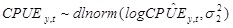
Different estimation models and survey designs may produce considerably different amounts of errors in the estimation of peak, lower, and upper days (Figs. 1-3). We were able to compare estimation errors more specifically in several aspects, namely in terms of absolute biases, variations, and mean absolute errors. In each aspect, comparisons were made in the following sequence: first, we compared performances of the three estimation models, SCPUE, hierarchical, and generalized additive (abbreviated as M1, M2, and M3, respectively). The same survey designs should be assumed unless otherwise specified when comparisons were made among estimation models. Second, we compared performances of 6-month relative to 12-month survey schemes. The same models and number of survey years should be assumed unless otherwise specified when comparisons were made between survey schemes. Third, we made comparisons within 6 and 12-month survey schemes. Finally, we examined the effect of different numbers of survey years on the estimation.
 |
Fig. (1). Errors in the estimation of the day (peak day) when annual abundance of soft shell crabs is the highest by the SCPUE model (1), the Hierarchical model (2), and the Generalized additive model (3). Five hundred data sets are obtained for each of the seven survey schemes with four different number of survey years. The red dot denotes the median over the five hundred estimates, and the two red bars and two blue dots indicate 5th and 95th percentiles and 25th and 75th percentiles, respectively. |
 |
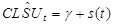
Fig. (2). Errors in the estimation of the day (lower day) which is earlier than the peak day and on which abundance of soft shell crabs is 85% of the abundance on the peak day by the SCPUE model (1), the Hierarchical model (2), and the Generalized additive model (3). Five hundred data sets are obtained for each of the seven survey schemes with four different number of survey years. The red dot denotes the median over the five hundred estimates, and the two red bars and two blue dots indicate 5th and 95th percentiles and 25th and 75th percentiles, respectively. |
3.1. Absolute Bias
Absolute biases in the estimation of peak day by M1 were, in most cases, either similar to or slightly lower than those by M2 (Fig. 4). However, absolute biases in the estimation of the lower or upper days by M1 were generally higher than M2, and the differences were particularly large for S6-12 (Figs. 5, 6). Absolute biases in the estimation of the peak, lower, or upper days by M3 were, in general, considerably lower than M1 or M2 (Figs. 4-6). Overall biases by M1 were generally higher than those by M2, except for S12-6 (Fig. 7).
Absolute biases in estimations of peak or upper days with 6-month survey schemes were lower than those with 12-month schemes (Figs. 4, 6). Absolute biases in the estimation of the lower day by M1 with these schemes were comparable to S11-12, S18-12, and S24-12 (Fig. 5). Absolute biases in estimations of the lower day by M1 were high with S6-12. Absolute biases in the estimation of the lower day by M2 were higher with the 6-month than 12-month survey schemes (Fig. 5). Overall biases were lower with the 6 month compared to 12 month schemes when M2 was applied (Fig. 7).
 |
Fig. (3). Errors in the estimation of the day (upper day) which is later than the peak day and on which abundance of soft shell crabs is 85% of the abundance on the peak day by the SCPUE model (1), the Hierarchical model (2), and the Generalized additive model (3). Five hundred data sets are obtained for each of the seven survey schemes with four different number of survey years. The red dot denotes the median over the five hundred estimates, and the two red bars and two blue dots indicate 5th and 95th percentiles and 25th and 75th percentiles, respectively. |
Absolute biases in the estimation of the peak, lower, or upper days, as well as overall biases, were either similar or lower when a survey scheme changed from S6-6 to S12-6 (Figs. 4-7). Increasing the number of sampling events in the 12-month survey schemes did not necessarily reduce biases. Absolute biases in the estimation of the peak or upper days by M1 or M2 were lower for S11-12 compared to S12-12, S18-12 or S24-12, and slightly lower for S18-12 compared to S12-12 or S24-12 (Figs. 4, 6). Absolute biases in the estimation of the lower day by M1 or M2 were more comparable among survey schemes S11-12, S12-12, S18-12, and S24-12 (Fig. 5). Overall biases were lower for S11-12 than for other 12-month survey schemes when M1 was used, and comparable among the 12-month survey schemes when M2 was used (Fig. 7).
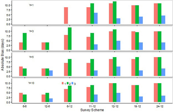 |
Fig. (4). Absolute values for biases (medians of errors) in the estimation of the peak day by the SCPUE model (1), the Hierarchical model (2), and the Generalized additive model (3) over seven survey schemes and four different number of survey years. |
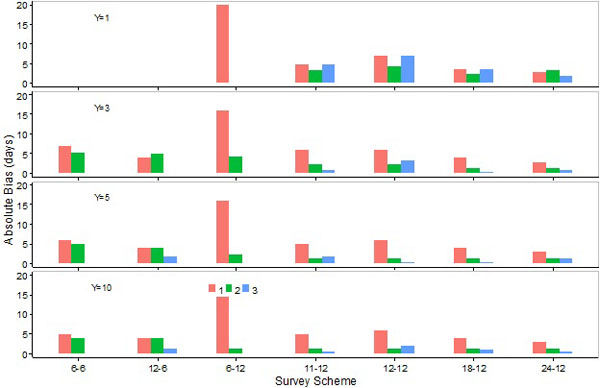 |
Fig. (5). Absolute values for biases (medians of errors) in the estimation of the lower day by the SCPUE model (1), the Hierarchical model (2), and the Generalized additive model (3) over seven survey schemes and four different number of survey years. |
Mean absolute biases decreased slightly when the number of survey years increased from 1 to 3, and remained virtually unchanged when the number of years increased beyond three (Fig. 8A).
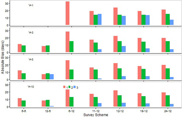 |
Fig. (6). Absolute values for biases (medians of errors) in the estimation of the upper day by the SCPUE model (1), the Hierarchical model (2), and the Generalized additive model (3) over seven survey schemes and four different number of survey years. |
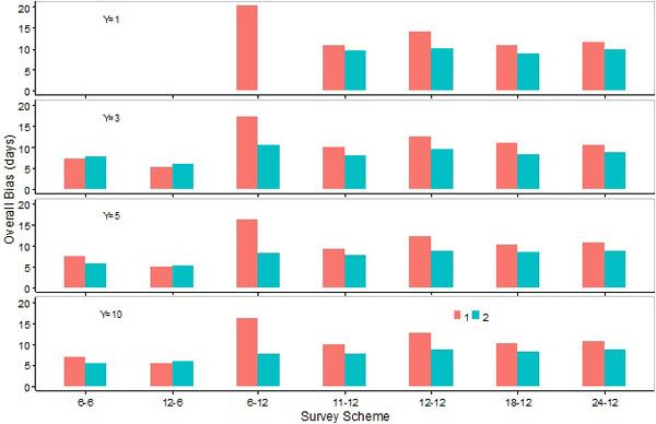 |
Fig. (7). Overall biases (averages of the absolute biases in the estimations of the peak, lower and upper days) for the SCPUE model (1) and the hierarchical model (2) over seven survey schemes and four different number of survey years.. |
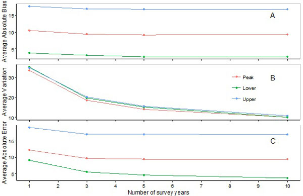 |
Fig. (8). Changes in averages of absolute biases (A), variations (B) and absolute errors (C) in the estimation of the peak, lower and upper days when the number of survey years increases. |
 |
Fig. (9). Variations (differences between 95th and 5th percentiles of the errors) in the estimation of the peak day by the SCPUE model (1), the Hierarchical model (2), and the Generalized additive model (3) over seven survey schemes and four different number of survey years. |
3.2. Variation
Variations in the estimation of the peak, lower, and upper days by M1 were, in general, similar to M2, and considerably lower than M3 (Figs. 9-11). Overall variations by M1 were generally similar to, or slightly higher than, those estimated by M2, except for S12-6 whereby M1 produced slightly lower overall variations when survey programs were 3 or 5 years long (Fig. 12).
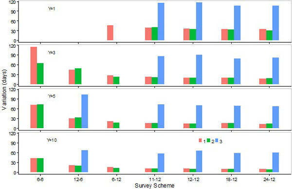 |
Fig. (10). Variations (differences between 95th and 5th percentiles of the errors) in the estimation of the lower day by the SCPUE model (1), the Hierarchical model (2), and the Generalized additive model (3) over seven survey schemes and four different number of survey years. |
Variations in the estimation of the peak, lower, and upper days, as well as overall variations, were higher for 6-month than 12-month survey schemes (Figs. 9-12). Differences increased when the number of survey years decreased from 10 to 5 or 5 to 3 (Figs. 9-12).
 |
Fig. (11). Variations (differences between 95th and 5th percentiles of the errors) in the estimation of the upper day by the SCPUE model (1), the Hierarchical model (2), and the Generalized additive model (3) over seven survey schemes and four different number of survey years. |
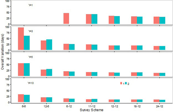 |
Fig. (12). Overall variations (averages of the variations in the estimations of the peak, lower and upper days) for the SCPUE model (1), and the hierarchical model (2) over seven survey schemes and four different number of survey years. |
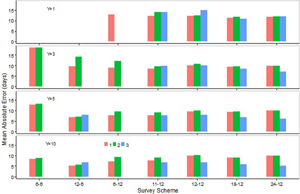 |
Fig. (13). Means of absolute values for errors in the estimation of the peak day by the SCPUE model (1), the Hierarchical model (2), and the Generalized additive model (3) over seven survey schemes and four different number of survey years. |
Variations in the estimation of the peak, lower, and upper days, as well as overall variations, were lower for S6-12 than S12-6 (Figs. 9-12). Variations in the estimation of the peak day by M1 or M2 were only slightly higher for S6-12 and S11-12 than S12-12, S18-12, and S24-12, and the differences decreased when the number of survey years increased (Fig. 9). Variations in the estimation of the lower or upper days, as well as the overall variation, decreased slightly when the number of sampling events increased for 12-month survey schemes (Figs. 10-12).
Mean variations decreased when the number of survey years increased. However, the extent of the decrease with one additional survey year declined when the number of survey years increased. The extent of the decrease was marginal with 5 survey years (Fig. 8B).
3.3. Mean Absolute Error
Mean absolute errors in the estimation of peak days by M1 were similar to, or slightly lower than, those estimated by M2, and such errors by M3 were generally lower than those by M1 or M2 except for sampling scheme S12-6 (Fig. 13). Mean absolute errors in the estimation of the lower or upper days by M1 were, in general, higher than those by M2 except for survey scheme S12-6 (Figs. 14, 15). Mean absolute errors in the estimation of the lower day by M3 were higher than those by M1 or M2 (Fig. 14). Mean absolute errors in the estimation of the upper day by M3 were generally higher than those by M2 (except when 10 years of data were collected), and lower than those by M1 except for S12-6 when 3 or more years of data were collected (Fig. 15). Overall errors were higher for M1 than M2, the exception being sampling scheme S12-6 (Fig. 16).
Mean absolute errors in the estimation of the peak or upper days by M1 or M2 were generally lower for S12-6 than for 12-month survey schemes (Figs. 13, 15). Mean absolute errors in the estimation of the lower day by M1 or M2 were, however, higher for S12-6 than 12 month schemes (Fig. 14). Overall errors were lower for S12-6 than 12-month survey schemes when data were collected for 5 or 10 years (Fig. 16). Mean absolute errors in the estimation of the peak or upper day by M1 or M2 were either similar or higher for S6-6 than 12-month survey schemes when data were collected for 3 or 5 years, and lower for the former scheme when data were collected for 10 years (Figs. 13, 15). Mean absolute errors in the estimation of the lower day by M1 or M2 were considerably higher for S6-6 than 12-month survey schemes (Fig. 14). Overall errors were generally higher for S6-6 than 12-month survey schemes (Fig. 16).
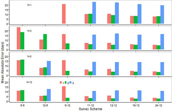 |
Fig. (14). Means of absolute values for errors in the estimation of the lower day by the SCPUE model (1), the Hierarchical model (2), and the Generalized additive model (3) over seven survey schemes and four different number of survey years. |
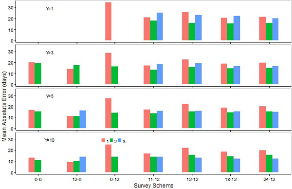 |
Fig. (15). Means of absolute values for errors in the estimation of the upper day by the SCPUE model (1), the Hierarchical model (2), and the Generalized additive model (3) over seven survey schemes and four different number of survey years. |
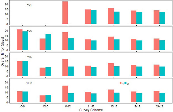 |
Fig. (16). Overall errors (averages of the absolute errors in the estimations of the peak, lower and upper days) for the SCPUE model (1) and the hierarchical model (2) over seven survey schemes and four different number of survey years. |
Mean absolute errors in the estimation of the peak, lower, and upper days, as well as overall errors, were lower for S12-6 than S6-6 (Figs. 13-16). Increasing the number of sampling events in 12-month survey schemes did not necessarily reduce mean absolute errors. Mean absolute errors in the estimation of the peak or upper days by M1 or M2 were, in general, slightly lower for S11-12 and S18-12 than S12-12 and S24-12. Mean absolute errors in the estimation of the lower day decreased slightly as the number of years increased in 12-month survey schemes (Figs. 13-15). When M2 was applied, overall errors were comparable among 12-month survey schemes (Fig. 16). In contrast, when M1 was applied overall errors were lower for S11-12 than other 12-month schemes, and such errors were noticeably higher for S6-12 (Fig. 16).
Mean absolute errors decreased when the number of years during which data were collected increased from 1 to 3, and remained relatively unchanged when the number of years increased beyond 3 (Fig. 8C).
At times the models produced very imprecise outputs. For instance, in most cases where the survey program lasted for only one year, ranges between the 5th and 95th percentiles of errors in the estimation of the peak day are well above 100 days. The generalized additive model also failed to produce sensible results for certain survey schemes, even when surveys were conducted during multiple years. These flawed outputs were not presented.
DISCUSSION
Simulation testing has often been used as an approach to evaluate performances of alternative stock assessment models [22, 23]. In simulation testing, data used by assessment models are generated from a simulation model with assigned parameter values believed to resemble reality as closely as possible. Therefore, the ‘true’ parameter values are known, enabling evaluation of assessment models’ estimation accuracies. However, outcomes of assessment model evaluations may rely on how the simulation model is specified [24]. When an assessment model is structurally similar to the operating model used to generate simulated data sets, then the assessment model should expectedly perform better on the simulation data compared to other competing models containing different features. In this simulation study, in order to avoid or mitigate evaluation biases due to structural similarity between operating and assessment models, we used a two-piece normal model to generate simulation data, as this operating model is substantially different from the three assessment models (SCPUE, hierarchical, and generalized additive).
Another challenge with simulation studies is the difficulty in determining whether the operating model generates realistic data [25]. The pattern of data generated in this study was based on results by Waddell et al. [9]. Softshell data generated from the two-piece normal model resembled the reported softshell pattern when the first day of a particular year was chosen to be in the autumn. This made the trend in softshell abundance versus time more symmetrical. To enhance the realism of simulated data, some random variations were incorporated into the data. Softshell crab abundance and peak moult time vary randomly among years, and moulting probability for any given day also has random variation. There is also a large amount of variation (59% coefficient of variation) in the survey data, imitating large observation errors in catch rate (CPUE) in the real world. We believe generated data realistically captured the essence of the true softshell pattern observed in BC waters for large male Dungeness Crabs.
In statistical analyses we often deal with random variables that are independent and identically distributed (iid). Estimation errors tend to decrease when the number of iid data increases. Although softshell data produced from crab surveys are independent, they are not from the same distribution because distributions of softshell crab abundance likely vary at two different sampling occasions. These data are, therefore, not direct measures of parameters of interest such as the peak softshell concentration or peak day, but rather they are used to construct a curve of relative abundance of softshell crabs on a daily basis from which the peak day and softshell period (which is approximately 2.5 months long) can be deduced and used in this simulation study. Estimation errors might not decrease when more sampling is conducted, especially in seasons with low softshell crab abundance.
Our simulation study comparatively evaluated the effectiveness of various survey designs, efficacies of different estimation models, and estimation stabilities for a varied number of survey years. The best survey design for collecting crab shell condition data in order to determine softshell periods is the survey scheme S11-12, closely followed by S6-12. However, since S6-12 would require less effort it is, therefore, likely more economical. In BC, surveys collecting Dungeness Crab softshell data are currently being conducted once every two months. This survey strategy is appropriate as it conforms to S6-12. The hierarchical model performed best, closely followed by the SCPUE model. The generalized additive model produced rather unstable estimations. We, therefore, recommend using the hierarchical model to estimate softshell periods, even though expected differences in outputs from the hierarchical model and the SCPUE model are not likely to be large. Data used by the models should be collected for, at least, three years. Unfortunately we were unable to find publications on similar studies and, consequently, were not able to compare our results. Nevertheless, our study provides baseline information for future research in this area.
CONFILICT OF INTEREST
The authors confirm that this article content has no conflict of interest.
ACKNOWLEDGEMENTS
We thank two reviewers for providing constructive comments, which helped to improve the quality of the manuscript.
REFERENCES
| [1] | Jensen G, Armstrong D. Range extensions of some Northeastern Pacific decapoda. Crustaceana 1987; 52: 215-7. |
| [2] | Jensen G. Pacific Coast Crabs and Shrimps. Monterey, CA: Sea Challengers 1995. |
| [3] | Butler TH. Maturity and breeding of the Pacific edible crab, Cancer magister, Dana. J Fish Res Bd Can 1960; 17: 641-6. |
| [4] | Butler TH. Growth and age determination of the Pacific edible crab, Cancer magister Dana. J Fish Res Bd Can 1961; 18: 873-91. |
| [5] | WDFW. Soft-shell Crab Identification.. Recreational Crab Fishing. Washington Department of Fish and Wildlife. 2015. Available from: http://wdfw.wa.gov/fishing/shellfish/crab/softshell.html [accessed 10 February]; |
| [6] | Tegelberg HC, Magoon D. Handling mortality on softshell Dungeness crab. In: Proceedings of the National Shellfisheries Association; Washington Department of Fisheries. 1971; pp. 13-4. |
| [7] | Tegelberg HC. Condition, yield, and handling mortality studies on Dungeness crabs during the 1969 and 1970 seasons. 23rd Annual Report of the Pacific Marine Fisheries Commission for the year 1970. Pacific Marine Commission; Portland, Oregon. 1972; pp. 42-7. |
| [8] | Kruse GH, Hicks D, Murphy MC. Handling increases mortality of softshell Dungeness crabs returned to the sea. Alaska Fishery Res Bull 1994; 1: 1-9. |
| [9] | Waddell B, Dunham JS, Zhang Z, Perry RI. Evaluation of soft-shell data for legal-sized male Dungeness Crabs (Metacarcinus magister) in Crab Management Areas E-S, E-T, G, and H in British Columbia. 2009-2013; DFO Can Sci Advis Sec Res Doc 2016/012.xii+110p. |
| [10] | Mohr M, Hankin D. Estimation of size-specific molting probabilities in adult decapod crustaceans based on postmolt indicator data. Can J Fish Aquat Sci 1989; 46: 1819-30. |
| [11] | Hankin D, Butler T, Wild P, Xue Q. Does intense fishing on males impair mating success of female Dungeness crabs? Can J Fish Aquat Sci 1997; 54: 655-69. |
| [12] | Shirley TC, Sturdevant M. Dungeness crab mating study. University of Alaska, Southeast, School of Fisheries and Science. In: Annual report to the Alaskan Department of Fish and Game, No. UASE; Juneau. 1988; pp. 87-20. |
| [13] | Rasmuson LK. The biology, ecology and fishery of the Dungeness crab, Cancer magister. Adv Mar Biol 2013; 65: 95-148. |
| [14] | Velasquez D, Burton S. Puget Sound Dungeness crab (Cancer magister) molting patterns. J Shellfish Res 2001; 20: 1198. |
| [15] | Velasquez DE, Burton SF, Sterritt DA, McLaughlin B. Shell condition testing of Dungeness crab in Puget Sound, Washington. J Shellfish Res 2003; 22: 609. |
| [16] | Zhang Z, Dunham JS. Construction of biological reference points for management of the Dungeness crab, Cancer magister, fishery in the Fraser River Delta, British Columbia, Canada. Fish Res 2013; 139: 18-27. |
| [17] | John S. The three-parameter two-piece normal family of distributions and its fitting. Commun Stat Theory Methods 1982; 11: 879-85. |
| [18] | R Core Team. A language and environment for statistical computing R Foundation for Statistical Computing, Vienna, Austria. 2015, Available from: https://www.R-project.org/. |
| [19] | Spiegelhalter D, Thomas A, Best N, Lunn D. WinBUGS Version 14 user manual. Cambridge: MRC Biostatistics Unit 2003. |
| [20] | Lunn D, Jackson C, Best N, Thomas A, Thomas A. The BUGS book: a practical introduction to Bayesian analysis. Boca Raton, FL: CRC Press 2013. |
| [21] | Gelman A, Rubin RB. Inference from iterative simulation using multiple sequences (with discussion). Stat Sci 1992; 7: 457-511. |
| [22] | Punt AE, Smith AD, Cui G. Evaluation of management tools for Australia’s south east fishery 2: how well can management quantities be estimated? Mar Freshw Res 2002; 53: 631-44. |
| [23] | Radomski P, Bence JR, Quinn TJ. Comparison of virtual population analysis and statistical kill-at-age analysis for a recreational, kill-dominated fishery. Can J Fish Aquat Sci 2005; 62: 436-52. |
| [24] | Butterworth DS, Rademeyer RA. Statistical catch-at-age analysis vs. ADAPT-VPA: the case of Gulf of Maine cod. ICES J Mar Sci 2008; 65: 1717-32. |
| [25] | Lehman RS. Computer simulation and modeling. New Jersey: Lawrence Erlbaum Associatiotes, Inc. 1977. |