
RESEARCH ARTICLE
Exploring the Biological Basis of Age-Specific Return Variability of Chinook Salmon (Oncorhynchus tshawytscha) From the Robertson Creek Hatchery, British Columbia Using Biological or Physical Oceanographic Explanatory Variables
R. W. Tanasichuk1, *, S. Emmonds2
Article Information

Identifiers and Pagination:
Year: 2016Volume: 9
First Page: 15
Last Page: 25
Publisher Id: TOFISHSJ-9-15
DOI: 10.2174/1874401X01609010015
Article History:
Received Date: 18/12/2014Revision Received Date: 17/09/2015
Acceptance Date: 17/09/2015
Electronic publication date: 30/04/2016
Collection year: 2016
open-access license: This is an open access article licensed under the terms of the Creative Commons Attribution-Non-Commercial 4.0 International Public License (CC BY-NC 4.0) (https://creativecommons.org/licenses/by-nc/4.0/legalcode), which permits unrestricted, non-commercial use, distribution and reproduction in any medium, provided the work is properly cited.
Abstract
We used information about hatchery rearing and release practices for 173 releases of age 0+ smolts between 1982 and 2012, as well as time series of early marine prey biomass and predator abundance/biomass, to investigate the biological basis of age-specific return variability of chinook salmon (Oncorhynchus tshawytscha) from the Robertson Creek Hatchery. We used survival rate as the response variable and considered the rate to be an apparent one because it is the product of the survival and maturation rates. Results of multiple regression analyses (adjusted R2 ranging between 0.43 and 0.59) showed that Pacific mackerel (Scomber japonicus) and Steller sea lion (Eumetopias jubatus) abundances accounted consistently for all of the explained variation in age-specific survival rate. We suggest that the persistence of the early marine (predation) effect with age shows that there is no effect of hatchery practice on age at maturity. Apparent survival rate variation was not explained when we used conventional physical oceanographic measurements (temperature, salinity, Pacific Decadal Oscillation Index, Northern Oscillation Index, Arctic Oscillation Index, Aleutian Low Pressure Index, Bakun Upwelling Index, timing of spring transition) in our analyses.
INTRODUCTION
Investigators have spent considerable effort exploring the basis of chinook salmon (Oncorhynchus tshawytscha) return variability. All studies (e.g. Sharma et al. [1], Miller et al. [2], Duffy [3], Scheuerell and Williams [4], Woodson et al. [5]) have implicitly focussed on the effects of food availability on size, with mortality resulting from predation (mis-mismatch hypothesis, see [6]; critical period hypothesis, see Cushing [7]; bigger is better hypothesis [8]) or the inability to store adequate energy reserves to survive the first winter at sea (critical size hypothesis, see [9]). These investigations used a variety of physical oceanographic measures as proxies for food. In addition, there are instances where size at ocean entry, influenced by freshwater or hatchery rearing, are also considered. The results suggest that the mortality during the early marine life history determines return variability.
The results of these studies are of concern to us for two reasons. The first one is that there is no empirical basis for relating physical oceanographic conditions directly to food availability. There are correlative relationships between physical oceanographic measures and zooplankton biomass (see Peterson et al. [10] for examples) but Tanasichuk and Routledge [11] and Tanasichuk et al. [12] found that juvenile salmon can select very specific parts of the zooplankton community as prey and correlative relationships at such fine taxonomic size scales have not been calculated. Wal- ters (cited in Coronado and Hilborn 1998 [13]) warned that the correlations between ocean condition and Oregon Production Index Area (OPI)coho (O. kisutch) production were spurious and consequently of no long term predictive value; the relationship between upwelling and OPI coho return described by Nicholson [14] has broken down. Myers [15] revisited 48 analyses that described correlative relationships between measures of aquatic conditions and recruitment and found that only one, for a fish population in a lake in Ontario, persisted. Scheuerell and Williams [4] noted that the correlations between North Pacific salmon production and oceanographic variables rarely lead to accurate predictions because the correlations degrade over time. Our second concern is about the statistical methodology. In all instances, there are a number of factors being tested and Bonferroni adjusted probabilities (see [16]) are not used to minimize the likelihood of committing a Type I experimental error. Tovey [17] is exceptional by her use of Bonferroni adjusted probabilities.
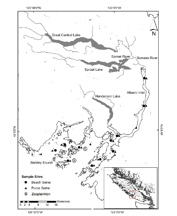 |
Fig. (1). Alberni Inlet and Barkley Sound showing fishing locations used to learn about hatchery chinook migration timing, distribution and diet, and zooplankton sampling stations used to monitor prey availability. A - Amphitrite Point lighthouse. Robertson Creek Hatchery is 2 km downstream of the outlet of Great Central Lake. |
We took advantage of multi decadal time series of information about rearing and release practices for chinook salmon from the Robertson Creek Hatchery, results of an investigation of the early marine life history of chinook from the Hatchery [12], and a multi decadal time series of prey availability and predator biomass/abundance during the early marine life history (the first marine summer), to test a number of null hypotheses regarding release specific return variability for the commonly returning ages of fish. We chose survival rate, the proportion of fish released that return or are caught at a given age, as the response variable because it is the product of the actual survival rate and the maturation rate; this survival rate is an apparent one. Variation in age at maturity may contribute to age specific return variability. Hankin et al. [18] found that age at maturity was heritable for males and females but suggested some plasticity as a consequence of growth variation. Wells et al. [19] reported that growth during the year before the return year affected the rate at which age 4 chinook from northern California matured. The apparent survival rate we used gave us the opportunity to consider survival and maturation simultaneously. The null hypotheses we tested were that there were no fish size at release, rearing density, the timing of release, the number of fish in a given release, the total number of fish released, and prey biomass and predator biomass/abundance during the early marine life history on the age specific survival rate of ages 2 through 5 chinook salmon from releases from the Robertson Creek Hatchery. We also took advantage of the opportunity to test the efficacy of physical oceanography measurements to explain variation in apparent age specific survival rate.
MATERIALS AND METHODOLOGY
Study Area and Early Marine Life History
The study area encompasses the Robertson Creek Hatchery and Alberni Canal/Barkley Sound Fig. (1) where fish are reared and spend the first two months of their marine life [12], and the West Coast of Vancouver Island (WCVI) (Fig. (1) inset map), which they would traverse to reach open ocean rearing areas. Fish are released into the Stamp River during the second half of May and travel 17 km to the Somass River estuary. Catches of hatchery chinook at the purse seining location closest to the estuary increase dramatically to a peak in mid June and decline rapidly subsequently. Fish persist in Barkley Sound until at least the end of August although catches decline in July. Hatchery chinook are distributed contagiously and catches are not correlated with those of any other species source (hatchery, wild) group. There is no diet overlap with any other species-source group. The diet is varied but euphausiids (Thysanoessa spinifera longer than 22 mm) appear to be persistent preferred prey in early July.
 |
Fig. (2). Robertson Creek Hatchery chinook rearing and release history, rearing density is kg • m-3. |
Data
Information about age 0+ smolt releases (1982-2012) and returns (1983-2013) was provided by the Canadian Department of Fisheries and Oceans' Salmonid Enhancement Programme (C. Lynch and J. Bateman, Fisheries and Ocean Canada, Vancouver, BC, pers. comm). Subsamples of all release groups were marked using release-specific coded wire tags. We used pond specific information on length (mm) and individual mass (g) at release, rearing density (kg · m3), number of fish liberated in a given release, day of year when release started as well as total number of fish released from the Hatcher y in a given year. Fig. (2) shows how pond specific fish size, rearing density, number of fish released, release date and total hatchery release have varied over time. Release specific return by age estimates were the sum of tag code expanded catches and escapement to the Hatchery. We excluded data for the 1990, 1994, 1996, 1997 brood years because tag codes could not be assigned to ponds unambiguously.
Information on prey availability for 1991-2012 was provided by a long-term monitoring programme of euphausiid/zooplankton productivity in Barkley Sound (see [20]). Biomass estimates (mg dry mass • m-2) were extracted for T. spinifera in July and for prey longer than 22 mm which was the size range selected by hatchery chinook. The sampling locations used for the monitoring programme are shown in Fig. (1).
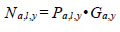
Information on predator abundance/biomass during the early marine life history came from a variety of sources. The hypothesis tests of the effects of predation and competition on return are based on observations for Barkley Sound/WCVI or described in the literature. Pacific hake (Merluccius productus) could prey on, or compete with, chinook smolts. Chinook smolts in Barkley Sound are the same size (~ 7 cm fork length) as Pacific herring consumed by hake, and hake occur in Barkley Sound in the summer [21]. Tanasichuk [22] reported that hake select T. spinifera longer than 17 mm which includes that part of the euphausiid biomass preferred by chinook smolts. There is a report of Pacific mackerel (Scomber japonicus) consuming chinook smolts in Barkley Sound. Results of a bi-weekly purse seine survey in Barkley Sound between April and July 1992 showed that Pacific mackerel were feeding intensively on hatchery chinook smolts. Preliminary calculations suggested that mackerel consumed that year’s production of chinook smolts from the Robertson Creek Hatchery (B. Patten, Fisheries and Oceans Canada, Pacific Biological Station, Nanaimo, BC. pers. comm.). There is no diet information for Steller sea lions (Eumetopias jubatus) for the WCVI. Steller sea lions consume salmon [23, 24] and appear to select salmon between 12 and 63 cm long [24]. We used the Regional Mark Information System (http://www.rmpc.org) and found that at least 80% of returning Robertson Creek Hatchery chinook were at least 65 cm long so we tested the effect of sea lion predation for the first marine year only. The information on Pacific hake biomass and Pacific mackerel abundance came from research mid water trawling along the WCVI (see [21]). We estimated year-specific total (planktivorous) and piscivourous biomasses of Pacific hake, the dominant fish species along the West Coast of Vancouver Island (WCVI) over the summer, using data from hydro-acoustic surveys (e.g. [25]) and biological sampling data from commercial and research mid water tows made off the WCVI. The hydro-acoustic surveys provided estimates of numbers of hake at age in Canadian waters. Age specific length frequencies were estimated from the sampling data and used to calculate age-specific numbers of fish at length from the survey estimates as follows:
 |
(1) |
where a is age, l is cm length interval, y is year, P is proportion, and G is number of fish estimated from the hydro-acoustic survey. Age, length and year specific biomass was estimated as:
 |
(2) |
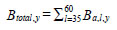
where m is estimated from year-specific length-mass regressions. Year-specific hake total biomass was estimated as:
 |
(3) |
. We used 1991-2005 hake diet data from fisheries oceanographic mid water trawl surveys along the WCVI in August to estimate the regression that described how the proportion of hake containing fish increased with predator size. A logit transformation [26] was applied to the proportion data so that the studentised residuals would be normally distributed. Results of an analysis of covariance showed no significant effect of year on the slope (p=0.11) and the intercept (p>0.05) based on the GT-2 multiple comparison test [26] of the year-specific regressions. The regression equation based on data pooled over years was:
 |
(4) |
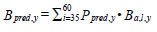
where L is the logit of the proportion of hake at a given length that could prey on fish (Ppred, l); the sample size is the number of year and cm length interval categories. Year-specific hake piscivorous biomass was estimated as:
 |
(5) |
Hydro-acoustic surveys were conducted annually between 1991 and 1998, in 2001 and 2003, and annually between 2005 and 2009. Abundance was interpolated linearly in years when there was no survey. We took advantage of time series of Steller sea lion abundances to consider their effect on Robertson Creek chinook salmon return. Abundances have been estimated intermittently between 1975 and 2006 [27], and in 2008, 2010 and 2013 (S. Majewski, Fisheries and Oceans Canada, Pacific Biological Station, Nanaimo, BC. pers. comm.) for locations including year-round haul-outs on the WCVI; abundance was extrapolated linearly for years when data were not collected. We used the location-specific abundances for our analyses as well as calculated sea lion abundance for the Southwest coast of Vancouver Island (Mara Rocks+Long Beach) and the Northwest coast of Vancouver Island (Oleary Rocks+Barrier Rocks+Solander Island).
Oceanographic data came from a number of sources. Monthly sea surface temperature and salinity data were extracted from http://www-sci.pac.dfo-mpo.gc.ca/osap/data/SearchTools/Searchlighthouse_e.htm for Amphitrite Point lighthouse (Fig. 1). Regional physical oceanographic indices included PDO (Pacific Decadal Oscillation; extracted from http://jisao.washington.edu/pdo/PDO.latest), NOI (Northern Oscillation Index; extracted from http://www.pfeg. noaa.gov/products/PFEL/modeled/indices/NOIx/noix_download.html), AO (Arctic Oscillation; extracted from http://www.cpc.ncep.noaa.gov/products/precip/CWlink/daily_ao_index/ao_index.html), the ALPI (Aleutian Low Pressure Index; extracted from http://www.pac.dfo-mpo.gc.ca/sci/sa-mfpd/climate/clm_indx_alpi.html), and the monthly mean upwelling indices for 48N 125W from (http://www.pfeg.noaa.gov/products/PFEL/modeled/indices/ upwelling/NA/data_download.html). We used daily upwelling indices from the same site to estimate the date of spring transition using the method described by Saitherwaite et al. [28].
Statistical Methods
Our analytical strategy was to try to learn about return variability at the age-specific level because this better reflected the complex age structure of Robertson Creek hatchery chinook and potentially provided insight about how hatchery practices may be affecting fish production by inadvertently affecting the age composition of returning fish. It is believed that Robertson Creek chinook become vulnerable to fishing only after they begin their return migration (G. Brown, Fisheries and Oceans Canada, Pacific Biological Station, Nanaimo BC, pers. comm.) so age-specific bias from removals should be minimal. We used the apparent survival rate (S) as the dependent variable where:
 |
(6) |
and C is expanded catch, E is expanded escapement to the Hatchery and R is the tag code-specific number of fish released from a pond; we used the logit of S in our analysis because the survival rate is a proportion. S is an apparent rate because it is the product of the marine survival and age-specific maturation rates.
We used stepwise multiple regression analysis to explore variation in the apparent survival rate as a function of hatchery rearing and release practices (size at release, rearing density, number of fish released either from the pond or the Hatchery, release day-of-the-year), and prey biomass and predator biomass/abundance during the early marine life history. The diagnostics used to accept a solution included ensuring there were no statistical outliers, the studentised residuals were normally distributed and there was no collinearity among the independent variables. We evaluated the significance of apparent outliers using the criteria suggests by Sokal and Rohlf [26]. Outliers were data pairs where |studentised residual|>2.5 and the leverage coefficient (h) was greater than 4•n-1, where n is the number of observations. The Variance Inflation Factor (VIF) was used to test for collinearity; VIF>5 indicated unacceptably high collinearity. Wilkinson et al. [16] noted that collinearity does not affect the predictive capability of the model, but the inflated standard errors of the parameter estimates makes the estimates suspect. We used the F-test that Sokal and Rohlf [26] recommended to test the significance of the increase in R2 associated with the inclusion of an additional independent variable. Standardised regression coefficients (β') were calculated for solutions based on more than one independent variable so that we could estimate the proportion of the explained variation accounted for by a specific independent variable. The proportion of explained variation accounted for by a given variable was calculated as the standardised regression coefficient for that variable divided by the sum of the standardised regression coefficients for all variables. Bonferroni adjusted probabilities were used to evaluate the significance of all models. Wilkinson et al. [16] recommended using Bonferroni adjusted probabilities to reduce the possibility of committing a Type I error when evaluating a number of relationships. The adjusted probabilities were estimated as:
 |
(7) |
where p is the critical value at α=0.05 at the appropriate degrees of freedom and c is the number of tests. We repeated the multiple regression analysis using information on time and size at release, rearing density, pond specific and total release and the physical oceanographic measures. We tested the effect of release date in relation to the spring transition by estimating the number of days after transition that the release took place.
RESULTS
We found that Pacific mackerel and sea lion abundance variability accounted for all of the explained variation in the apparent age and pond specific survival rate of ages 2 through 5 chinook salmon released as age 0+ smolts from the Robertson Creek Hatchery. The VIF’s indicated that the independent variables were not correlated. There was one outlier each for the initial regression tests of the effects of Pacific mackerel and sea lion abundances on logit survival rate of ages 4 or 5 fish; these were excluded before the solutions were calculated. The statistics for the regression analyses are presented in Table 1. Sea lion abundance at the NWCVI haul out sites accounted for 65, 74, 79, and 71% respectively of the explained variation in apparent survival rate for ages 2 through 5 Robertson Creek Hatchery chinook. Plots of predicted age-specific survival rates against observed pond specific rates are shown in Fig. (3).
Statistics for multiple regression explaining Robertson Creek Hatchery chinook age and pond specific return variability using empirical descriptions of prey and predator variability. padj=0.05•153-1=3.27E-04. NWCVI- Northwest coast Vancouver Island.
| Parameter | Estimate | Std. Error | p | β | VIF |
|---|---|---|---|---|---|
| Age 2; Adj. R2=0.49; p=1.24E-21; n=144 | |||||
| Intercept | -6.591 | 0.1726 | 3.02E-76 | 0 | |
| Pacific mackerel CPUE | -0.482 | 0.0792 | 1.01E-08 | -0.37 | 1.04 |
| NWCVI sea lion abundance | -0.001 | 0.00001 | 7.15E-21 | -0.68 | 1.04 |
| Age 3; Adj. R2=0.43; p=3.10E-17; n=133 | |||||
| Intercept | -4.522 | 0.1696 | 3.18E-55 | 0 | |
| Pacific mackerel CPUE | -0.295 | 0.0840 | 6.15E-04 | -0.23 | 1.03 |
| NWCVI sea lion abundance | -0.001 | 0.00001 | 7.91E-18 | -0.66 | 1.03 |
| Age 4; Adj. R2=0.59; p=1.38E-25; n=129 | |||||
| Intercept | -3.857 | 0.1159 | 2.91E-64 | 0 | |
| Pacific mackerel CPUE | -0.394 | 0.0522 | 7.65E-12 | -0.43 | 1.04 |
| NWCVI sea lion abundance | -0.001 | 0.00001 | 4.99E-24 | -0.72 | 1.04 |
| Age 5; Adj. R2=0.59; p=2.30E-24; n=122 | |||||
| Intercept | -4.776 | 0.1488 | 1.87E-60 | 0 | |
| Pacific mackerel CPUE | -0.430 | 0.0712 | 1.86E-08 | -0.36 | 1.03 |
| NWCVI sea lion abundance | -0.002 | 0.00001 | 5.58E-24 | -0.75 | 1.03 |
 |
Fig. (3). Observed (open circles) and predicted (closed circles) survival rates. |
There were no statistically significant solutions when we repeated the regression analyses using physical oceanographic measurements as explanatory variables.
DISCUSSION
Our tests of hatchery practice, prey and predator abundance/biomass effects suggested that return variability for ages 2 through 5 chinook from the Robertson Creek Hatchery is a consequence of predation with no effect of hatchery rearing or release practices, or prey variability. We note that, based on the results of a cluster analysis of survival rate (see [13]), Robertson Creek Hatchery chinook survival rate trends differ from those of Washington and Oregon populations that have been studied; there are no previous studies of survival variation for other Canadian chinook populations. The inability to explain survival rate variability using the physical oceanographic variables suggests that these variables are not accurate proxies, or reflect different processes for other chinook populations. The recurring conclusion of other studies (e.g. [5]) is that there is a relationship between local SST and survival for Pacific Northwest (Oregon to Alaska) chinook populations. It would be interesting to revisit previous explanations of return variability which are based on physical oceanographic variables to see if the results persist or fail as described in [15].
This study is the most comprehensive analysis of hatchery chinook return variability to date because it considers hatchery and early marine biological effects explicitly and simultaneously. Quiñones et al. [29] investigated the effects of hatchery release practices and some freshwater and oceanographic conditions on the return of salmonids to the Klamath River Basin, California. They reported that fall chinook returns were affected mostly by hatchery practices and that the spring and fall chinook populations were also affected by climatic effects (upwelling, summer river flows). Somewhat related, Haeseker et al. [30] noted that freshwater and marine survival rates of Snake River chinook were correlated.
We are intrigued by finding no effect of hatchery rearing or release practices because it contributes to the ongoing discussion about whether the hatchery affects return; as shown in Fig. (2), rearing and release conditions varied substantially during our study period. Results of previous experiments of the effect of time and size at-release (e.g. [31, 32]) showed that survival was affected more by release date than release size. However, Irvine et al. [33], based on 25-27 years of data, concluded more recently that the declining trend in survival of Strait of Georgia coho could not be reversed by manipulating release time and/or size as suggested by the results of the aforementioned short-term experiments. These authors also reported mixed effects of time and size at release among the five hatchery populations they examined. The results presented in [33] are unique because studies of hatchery effects on return are generally short term ones. Mathews and Ishida [34] using experiments conducted at a Columbia River hatchery for one brood year and a southern Oregon hatchery in the next brood year, found that the effect release size on coho survival were mixed. Burgess and Skalski [35] explored the basis of survival variability for fall chinook salmon released from 10 hatcheries along the Washington or Oregon coasts. They used coded wire tag release and return data for between 11 and 20 years. The authors reported mixed results for the effect of weight at release on the survival and that survival rate increased with date of release until September. Chittenden et al. [36] found that smolt to adult survival of coho released from the Quinsam River Hatchery, British Columbia peaked when fish were released at the time of the seasonal peak of zooplankton abundance. Duffy [3] reported that marine survival of coded-wire tagged release groups of juvenile chinook in Puget Sound was dependent on size in July of the first marine year so declines in marine survival since the 1980’s could be a result of reduced food availability in May and June; she found that release size and release date had a minor positive effect on survival. Duffy noted that the lack of an effect of fish size at release may be due to the small range (5-11 g) of mass at release. Quinn et al. [37] reported that, based on release sizes ranging between 3 and 20 g, intra-annual variations in marine survival were greater for heavier fish but fish size did not explain inter-annual survival variations. Tomaro [38] found, over an eight year study, that the return of adult mid upper Columbia River spring chinook was best explained by size of yearling smolts at ocean entry. Banks and LaMotte [39] found that rearing density had a minor, inconsistent effect on smolt to adult survival. Olsen and Paiya [40] reported mixed effects of lower density on adult survival; however they thought their low, medium and high experimental densities would all be considered to be low rearing densities. They, and [41], suggested that lower rearing densities enhanced survival when ocean conditions were poor. Bilton [32] reported a strong and positive curvilinear relationship between mass at release and return for chinook reared at the Big Qualicum Hatchery in the Strait of Georgia.
We found that no hatchery practice we tested explained variation in age at return. Ricker [42] reported that age at maturity of chinook is highly heritable and that age at maturity of males and females is, to some extent, determined by the sex of the parent. Hankin et al. [18] found that, in wild chinook experiments at the Elk River Hatchery, Oregon, heritability in age at maturity was relatively high, age at maturity of females was independent of age of the male parent, faster growing progeny for a given parental age matured at younger ages, and that size-at-age of progeny from older parents is not smaller. They concluded that age at maturity is not a function of growth rate. They proposed that there are heritable minimum threshold lengths that differentially trigger maturation as a consequence of parental age and sex. Wells et al. [19] explored environmental effects on at maturity of age 4 Northern California chinook. They found that accelerated growth in the third rather than the fourth year of life, as a consequence of physical oceanographic factors (negatively with spring sea level height, SST and scalar winds, and positively to curl, upwelling and northerly wind stresses), increased the likelihood of fish returning as 4 year olds. These authors stressed that their results do not imply cause and effect. Sharma [43] reported no link between age at maturity and ocean conditions for 23 populations of Pacific Northwest chinook salmon.
CONCLUSION
We conclude that predation explained the variation in return variability of ages 2 through 5 chinook salmon to the Robertson Creek Hatchery and there was no effect of the aspects of hatchery practice we tested on survival rate or age at maturity. Physical oceanographic variables did not provide an explanation for survival variation. We suggest that return variation of Robertson Creek Hatchery chinook is under biological control and hatchery practice modifications would have no influence on fish production.
CONFLICT OF INTEREST
The authors confirm that this article has no conflicts of interest.
ACKNOWLEDGEMENTS
We thank Westcoast Aquatic and the National Fish and Wildlife Foundation for their logistic and financial support. Special thanks to Kevin Bilton for his data mining efforts and to Cheryl Lynch and Joan Bateman for providing release and return data. Very special thanks go to Erin Vang, of Global Pragmatica, whose programming work made the evaluation of physical oceanographic variables possible.
REFERENCES
| [1] | Sharma R, Vélez-Espino LA, Wertheimer AC, Mantua N, Francis RC. Relating spatial and temporal scales of climate and ocean variability to survival of Pacific Northwest Chinook salmon (Oncorhynchus tshawytscha). Fish Oceanogr 2013; 22: 14-31. |
| [2] | Miller JA, Teel DJ, Baptista A, Morgan CA. Disentangling bottom-up and top-down effects on survival during early ocean residence in a population of Chinook salmon (Oncorhynchus tshawytscha). Can J Fish Aquat Sci 2013; 70: 617-29. |
| [3] | Duffy E. Factors during the early marine life that affect smolt to adult survival of ocean-type Puget Sound Chinook salmon (Oncorhynchus tshawytscha). PhD thesis, University of Washington. 2009. |
| [4] | Scheuerell MD, Williams JG. Forecasting climate-induced changes in the survival of Snake River spring/summer Chinook salmon (Oncorhynchus tshawytscha). Fish Oceanogr 2005; 14: 448-57. |
| [5] | Woodson LE, Wells BK, Weber PK, MacFarlane RB, Whitman GE, Johnson RC. Size, growth, and origin-dependent mortality of juvenile Chinook salmon Oncorhynchus tshawytscha during early ocean residence. Mar Ecol Prog Ser 2013; 487: 163-75. |
| [6] | Cushing DH. Plankton production and year-class strength in fish populations: an update of the Match/Mismatch hypothesis. Adv Mar Biol 1990; 26: 249-93. |
| [7] | Cushing DH. In: Cushing DH, Walsh JJ, Eds. The ecology of the seas. W.B. Saunders 1975; pp. 317-40. |
| [8] | Miller TJ, Crowder LB, Rice JA, Marschall EA. Larval size and recruitment mechanisms in fishes: toward a conceptual framework. Can J Fish Aquat Sci 1988; 45: 1657-70. |
| [9] | Beamish RJ, Mahnken C. A critical size and period hypothesis to explain natural regulation of salmon abundance and the linkage to climate and climate change. Prog Oceanogr 2001; 49: 423-37. |
| [10] | Peterson WT, Hooff RC, Morgan CA, Hunter KL, Casillas E, Ferguson JW. Ocean conditions and salmon survival in the northern California current. Available from: http://www.nwfsc.noaa.gov/research/divisions/fed/ecosysrep.pdf. 2006. |
| [11] | Tanasichuk RW, Routledge RD. An investigation of the biological basis of return variability for sockeye salmon (Oncorhynchus nerka) from Great Central and Sproat lakes, Vancouver Island. Fish Oceanogr 2013; 20: 462-78. |
| [12] | Tanasichuk RW, Grayson J, Yakimishyn J, Taylor S, Dagley GD. The early marine biology of the hatchery/wild juvenile salmonid (Oncorhynchus sp.) community in Barkley Sound, Canada. Open Fish Sci J 2014; 7: 8-22. |
| [13] | Coronado C, Hilborn R. Spatial and temporal factors affecting survival of coho and fall chinook salmon in the Pacific Northwest. Bull Mar Sci 1998; 62: 409-25. |
| [14] | Nickelson TE. Influences of upwelling, ocean temperature, and smolt abundance on marine survival of coho salmon (Oncorhynchus kisutch) in the Oregon production area. Can J Fish Aquat Sci 1986; 43: 527-35. |
| [15] | Myers RA. When do environment-recruitment correlations work? Rev Fish Biol Fish 1998; 8: 285-305. |
| [16] | Wilkinson L, Blank G, Gruber C. Desktop data analysis with SYSTAT. Upper Saddle River, NJ: Prentice-Hall Inc 1996. |
| [17] | Tovey CP. Evidence for inheritance of age of maturity in chinook salmon (Oncorhynchus tshawytscha). Can J Fish Aquat Sci 1993; 58: 347-58. |
| [18] | Hankin DG, Nicholas JW, Downey TW. Evidence for inheritance of age of maturity in chinook salmon (Oncorhynchus tshawytscha). Can J Fish Aquat Sci 1993; 58: 347-58. |
| [19] | Wells BK, Grimes CB, Waldvogel JB. Quantifying the effects of wind, upwelling curl, sea surface temperature, and sea level height on growth and maturation of a California Chinook salmon (Oncorhynchus tshawytscha) population. Fish Oceanogr 2007; 16: 363-82. |
| [20] | Tanasichuk RW. Interannual variations in the population biology and productivity of the euphausiid Thysanoessa spinifera in Barkley Sound, Canada, with special reference to the 1992 and 1993 warm ocean years. Mar Ecol Prog Ser 1998; 173: 163-80. |
| [21] | Tanasichuk RW, Ware DM, Shaw W, McFarlane GA. Variations in the diet, daily ration and feeding periodicity of Pacific hake (Merluccius productus) and spiny dogfish (Squalus acanthias) off the lower west coast of Vancouver Island. Can J Fish Aquat Sci 1991; 48: 2118-28. |
| [22] | Tanasichuk RW. Interannual variation in the availability of euphausiids as prey for Pacific hake (Merluccius productus) along the southwest coast of Vancouver Island. Fish Oceanogr 1999; 8: 150-6. |
| [23] | Trites AW, Calkins DG, Winship AJ. Diets of Steller sea lions (Eumetopias jubatus) in Southeast Alaska, 1993-99. Fish Bull 2007; 105: 234-48. |
| [24] | Stigler MF, Tollit DJ, Vollenweider JJ, et al. Steller sea lion foraging response to seasonal changes in prey availability. Mar Ecol Prog Ser 2009; 388: 243-61. |
| [25] | Fleischer GW, Cooke KD, Ressler PH, et al. The 2003 integrated acoustic and trawl survey of Pacific hake, Merluccius productus, in U. S. and Canadian waters off the Pacific Coast. NOAA Technical Memo, 2005; NMFS-NWFSC-65: p. 61.. |
| [26] | Sokal RR, Rohlf FJ. Biometry: The principles and practice of statistics in biological research. 3rd ed. New York: W. H. Freeman and Company 2003. |
| [27] | Olesiuk PF. Abundance of Steller sea lions (Eumetopias jubatus) in British Columbia. Can Sci Advis Res Doc, 2008; 2008/63 p .33. |
| [28] | Satterthwaite WH, Carlson SM, Allen-Moran SD, Vincenzi S, Bograd SJ, Wells BK. Match-mismatch dynamics and the relationship between ocean-entry timing and relative ocean recoveries of Central Valley fall run Chinook salmon. Mar Ecol Prog Ser 2014; 511: 237-48. |
| [29] | Quiñones RM, Holyoak M, Johnson ML, Moyle PB. Potential factors affecting survival differ by run-timing and location: linear mixed-effects models of Pacific salmonids (Oncorhynchus spp.) in the Klamath River, California. PLoS One 2014; 9(5): e98392. |
| [30] | Haeseker S, McCann JA, Tuomikowski J, Chockley B. Assessing freshwater and marine environmental influences on life-stage-specific survival rates of snake river spring-summer chinook salmon and steelhead. Trans Am Fish Soc 2012; 141: 121-38. |
| [31] | Bilton HT, Alderdice DF, Schnute JT. Influence of time and size at release of juvenile coho salmon (Oncorhynchus kisutch) on returns at maturity. Can J Fish Aquat Sci 1982; 39: 426-47. |
| [32] | Bilton HT. Return of Chinook Salmon in Relation to Juvenile Size at Release. Can Tech Rep Fish Aquat Sci 1984; 1245: 41p. |
| [33] | Irvine JR, O’Neill M, Godbout L, Schnute J. Effects of smolt release timing and size on the survival of hatchery-origin coho salmon in the Strait of Georgia. Prog Oceanogr 2013; 115: 111-8. |
| [34] | Mathews S, Ishida Y. Survival, ocean growth, and ocean distribution of differentially time releases of hatchery coho salmon (oncorhynchus kisutch). Can J Fish Aquat Sci 1989; 46: 1216-26. |
| [35] | Burgess C, Skalski J. Design and analysis of Salmonid Tagging Studies in the Columbia Basin,Volume XVII, Project No. 1991-005100. BPA Report DOE/BP-91572-8 2001; p. 155. |
| [36] | Chittenden CM, Jensen JL, Ewart D, et al. Recent salmon declines: a result of lost feeding opportunities due to bad timing? PLoS One 2010; 5(8): 312423. |
| [37] | Quinn TP, Dickerson BR, Vøllestad LA. Marine survival and distribution patterns of two Puget Sound hatchery populations of coho (Oncorhynchus kisutch) and chinook (Oncorhynchus tshawytscha). Fish Res 2005; 76: 209-20. |
| [38] | Tomaro LM. Effects of four density levels on Tule Fall Chinook Salmon during hatchery rearing and after release. North Amer J Aquacul 2002; 64: 24-33. |
| [39] | Miller JA. Year-class regulation of Mid-upper Columbia River Spring Chinook Salmon Oncorhynchus tshawytscha: The role of juvenile size, growth and migratory behaviour. MSc thesis, Oregon State University 2010. |
| [40] | Olsen DE, Paiya M. An evaluation of rearing densities to improve growth and survival of hatchery spring chinook salmon. J Fish Wildl Manage 2013; 4: 114-23. |
| [41] | Ewing RD, Ewing SK. Review of the effects of rearing density on survival to adulthood for Pacific salmon. Prog Fish Cult 1995; 57: 1-15. |
| [42] | Ricker WE. Heredity and environmental factors affecting certain salmon populations. The stock concept in Pacific salmon. In: H. R. MacMillan Lectures in Fisheries; University of British Columbia. 1972; pp. 19-160. |
| [43] | Sharma S. Ocean Distribution and Recruitment of Pacific Northwest Chinook Salmon (Oncorhynchus tshawytscha) in Relation to Environmental Factors, and Implications for Management. PhD thesis University of Washington. 2009. |